If you ever used Microsoft Excel, you know it’s a powerful tool. From beginners to math experts, everyone can find it useful. And when we say everyone, we also think of lottery players. Excel is also useful to create lottery strategies and algorithms to randomly generate numbers for your lottery entry.
Let’s clarify something – you don’t need any math or Excel knowledge to create this algorithm. Our experts created a beginner-friendly guide with a quick and fun way to use this lotto prediction utility. Check out what you need to know about lottery prediction algorithms and find step-by-step instructions for creating them below!
Key Takeaway
- Excel is beginner-friendly, so you don’t need advanced math or excel skills to create a lottery prediction algorithm.
- The Excel-based algorithm is customizable to various lottery games. You only need to adjust the initial range of numbers based on the specific lottery rules.
- Excel can also be used to calculate the probability of winning a lottery, letting you understand your odds of success for different games, including those with multiple drums.
- Excel-based algorithms do not guarantee a win. They only make it easier to choose your numbers.
Contents
How Does the Lottery Prediction Algorithm Work?
A lottery prediction algorithm is an algorithm that uses a large collection of numbers to help you pick the right lotto combination. You could explain it like this – you issue a command to Microsoft Excel (or another program) to analyze thousands (or millions) of numbers. Based on that analysis, the algorithm predicts the numbers that are most likely to show in that sequence.
You can use excel prediction algorithms for virtually any lottery out there. It can help you to choose numbers for a standard ticket, but also advanced play systems. Many prefer it to lottery strategies because algorithms are fun, free, and easy to use. .
However, the critical thing to note is that lottery prediction algorithms won’t guarantee a win. Remember that the lottery is a game of chance, so no lottery strategy or algorithm can accurately generate the lottery numbers before the draw. You only win through pure luck.
How to Create a Lottery Prediction Algorithm in Excel
It’s possible to find many videos with instructions on how to design lottery prediction algorithms. You don’t need any advanced Excel skills to create them. Furthermore, it’s more than enough to have that software and follow our guide. Here is how you can use this algorithm to choose the numbers for your upcoming session.
Prepare the Document
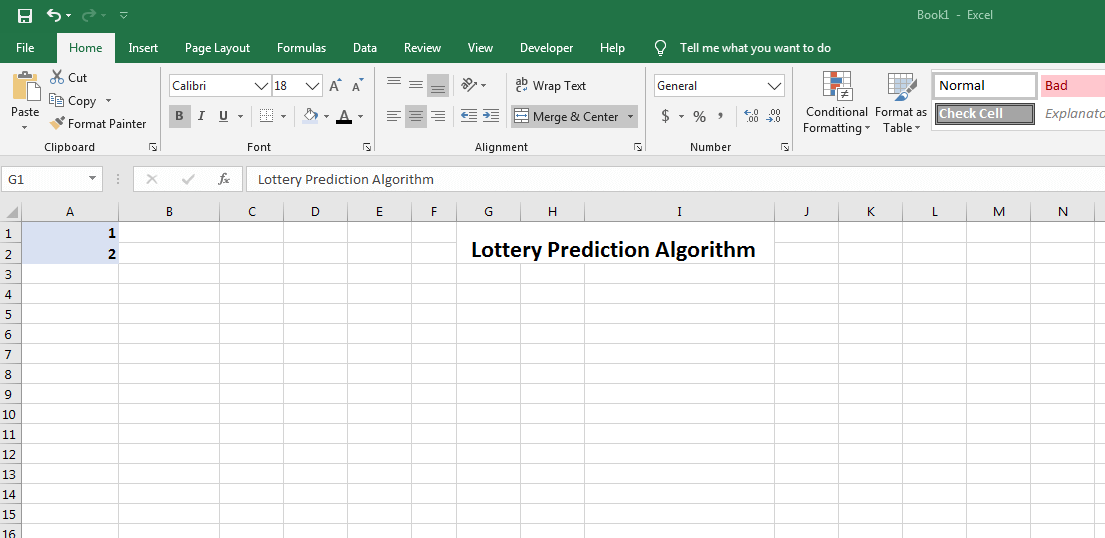
The first step is to open a blank document in your MS Excel. It’s up to you whether you want to save it. You can also consider making it more attractive by adding a title or choosing different colors for various columns.
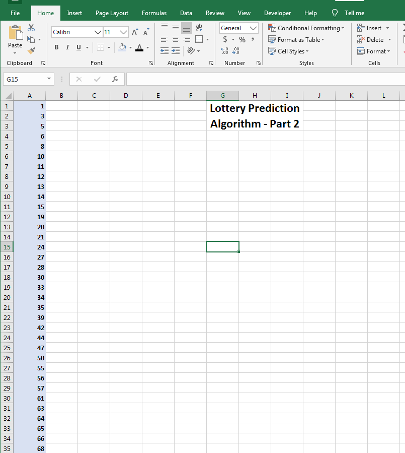
For now, the important thing is to leave the A and B cell rows free. Furthermore, the first thing you will do is to write down “1” in the “A1” cell and “2” in the “A2” cell. We also bolded and colored the cells for fun.
Fill the First Row Based on the Selected Lottery
Here is a crucial explanation – you can use this lottery prediction for any lotto game out there. However, you want to pick the lottery before you start. In this example, we’ll choose US Powerball since it’s one of the lotteries with the biggest jackpots in the world.
Now, the specific thing about the Powerball is that its main drum contains 69 balls. That’s why we will fill the first row until the column number “69.” You do this by using the little square that appears once you mark both “A1” and “A2” cells.
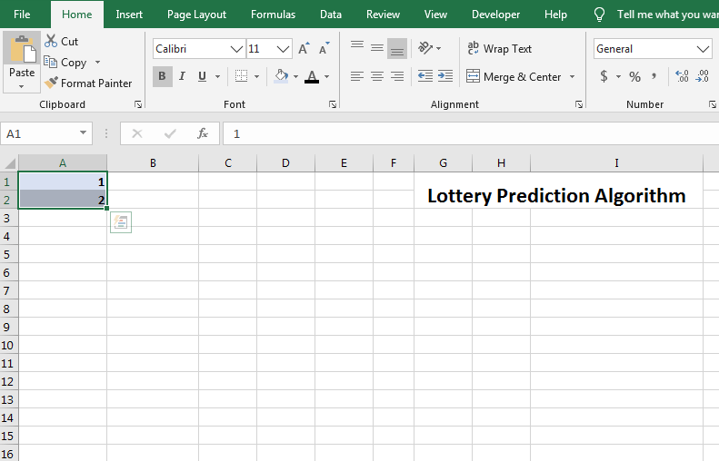
You want to pull that square downwards up until the 69th column (where you should see number 69).
If you want to play a different lottery, use the total number of balls in the main drum instead of “69.” For example, Canada Lotto 6/49 will require filling the first row only until the 49th column.
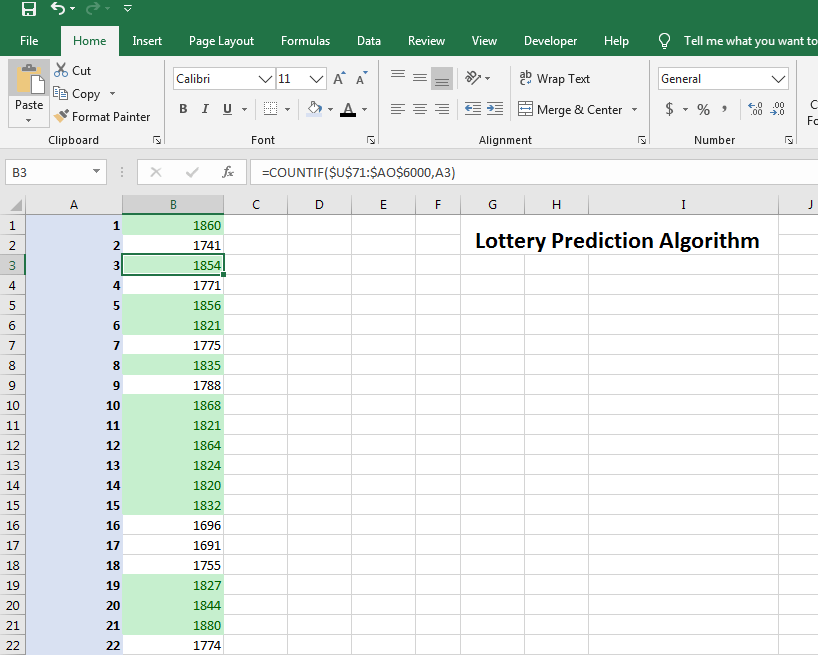
Enter the Function in B1 Cell
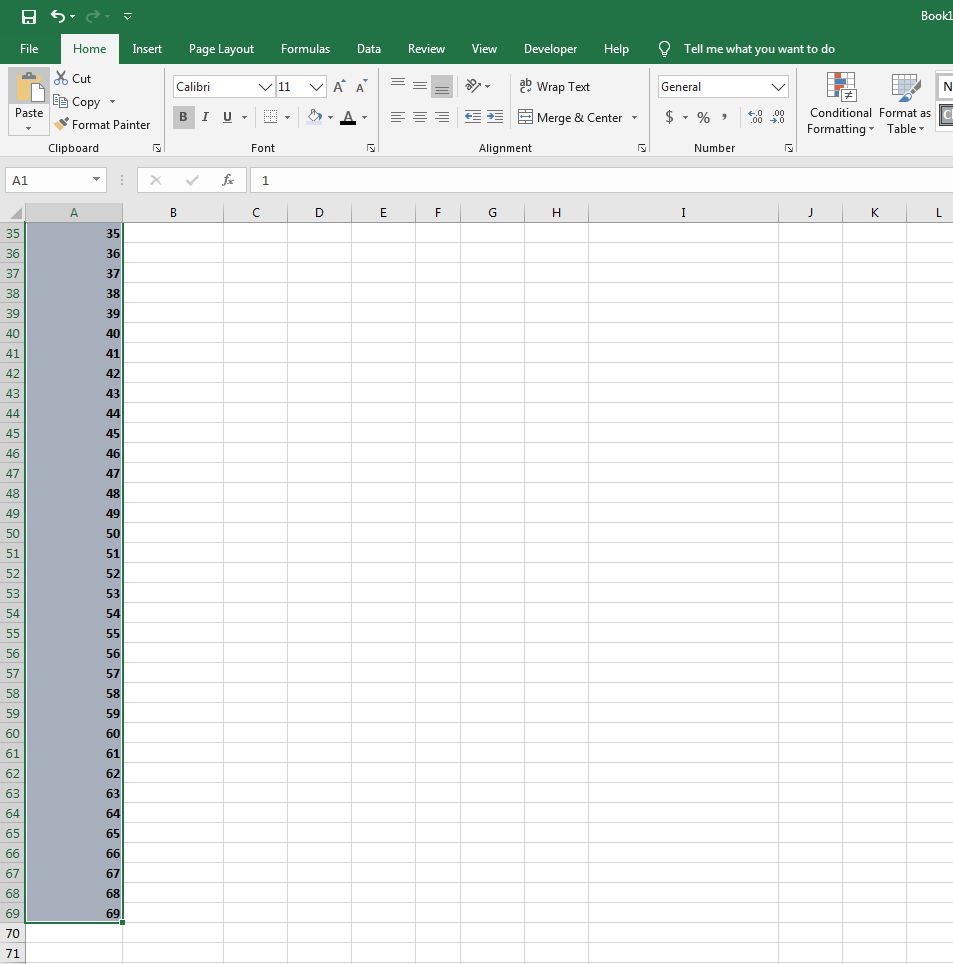
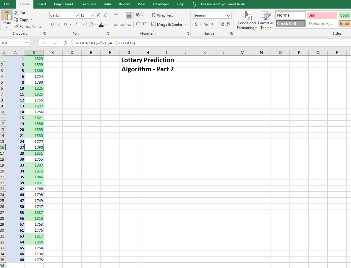
It’s now time to add a function that will help us to predict the numbers for the upcoming draw. We start by using the “B1” cell where you want to enter the following function:
=COUNTIF($U$71:$AO$6000,A1)
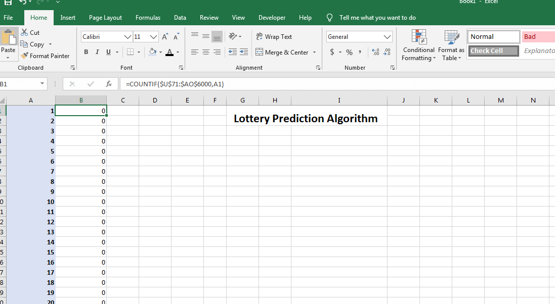
For those who know a thing or two about Excel, we made the cells absolute by using the “$” signs. Next, you want to use the little square in the bottom right section to apply this function to the entire B-row. That is all the way to the 69th column, which is where our lotto numbers end.
If you did everything right, the values should be “0” in the B column, but they’ll change later.
Now, select the entire B range, so cells between B1 and B69. Choose Conditional formatting at the top ribbon and select Top/Bottom Rules. Click on Above Average.
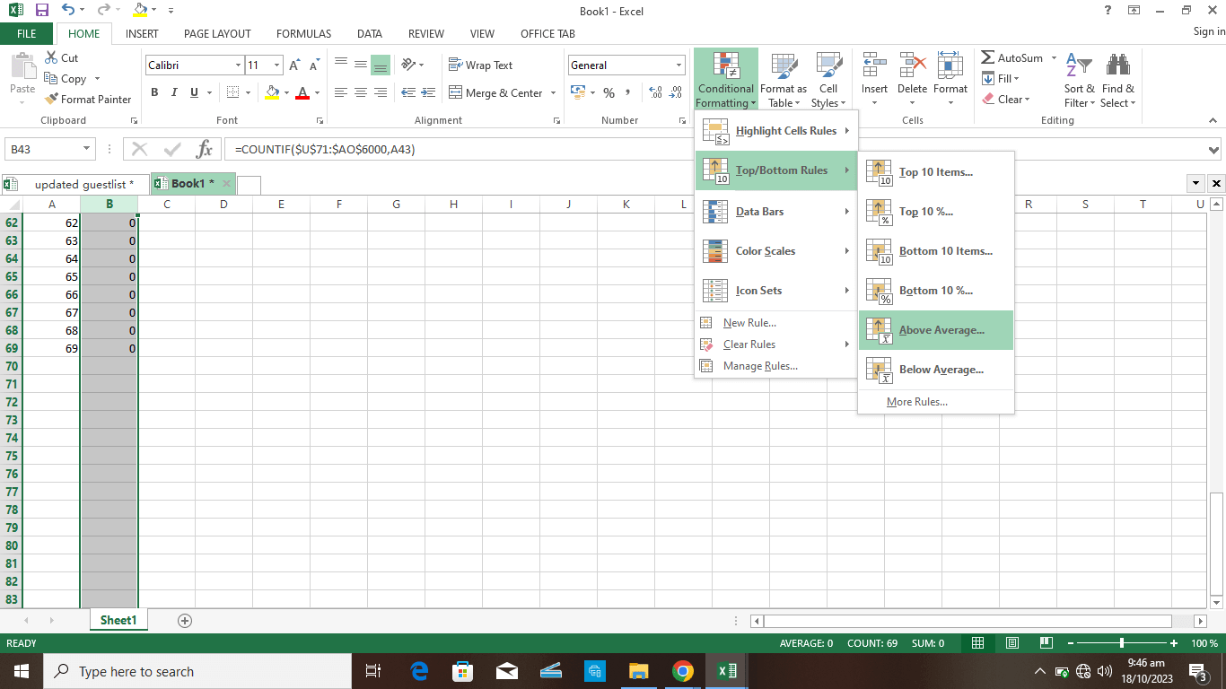
The idea is to highlight the cells with numbers that appear above average in our prediction algorithm. You can pick the desired highlighting option from the available ones.
Time for Another Function
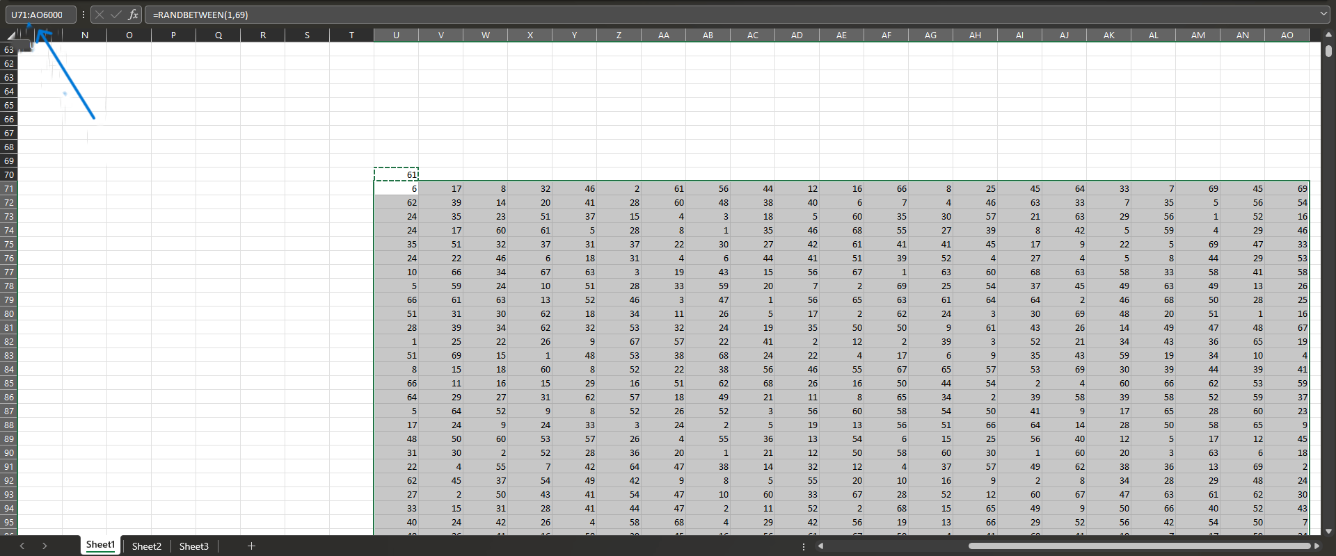
Our next step takes us all the way to cell “U70.” Mark that cell and enter the following function:
=RANDBETWEEN (1,69)
The function displays a random number from “1” to “69” in that cell. As you can notice, those are the numbers in the Powerball primary drum.
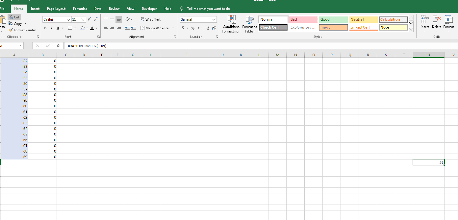
We got “56” in that particular cell, but the odds say you’ll get another number in this range, and that’s perfectly normal. Now, take a look at the reference box right above the “A” row. Copy the U70 cell by marking it and using “CTRL+C” on your keyboard.
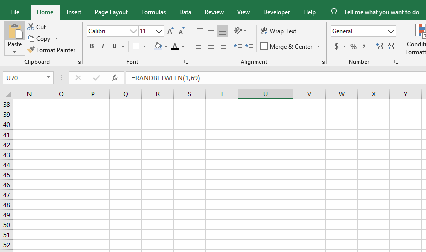
You’ll notice that it says “U70” here, but you want to type the following:
U71:AO6000
That will select a large number of cells in your document. Now, right-click on any of the selected cells and click on Paste Formulas.
You’ll see random numbers from 1 to 69 appearing in all those cells.
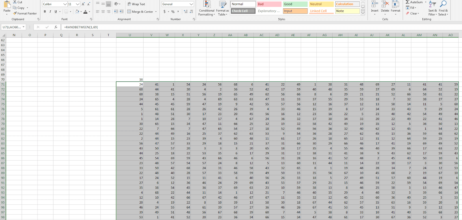
You now have more than 120,000 random numbers in these cells.
Copy the Random Combinations
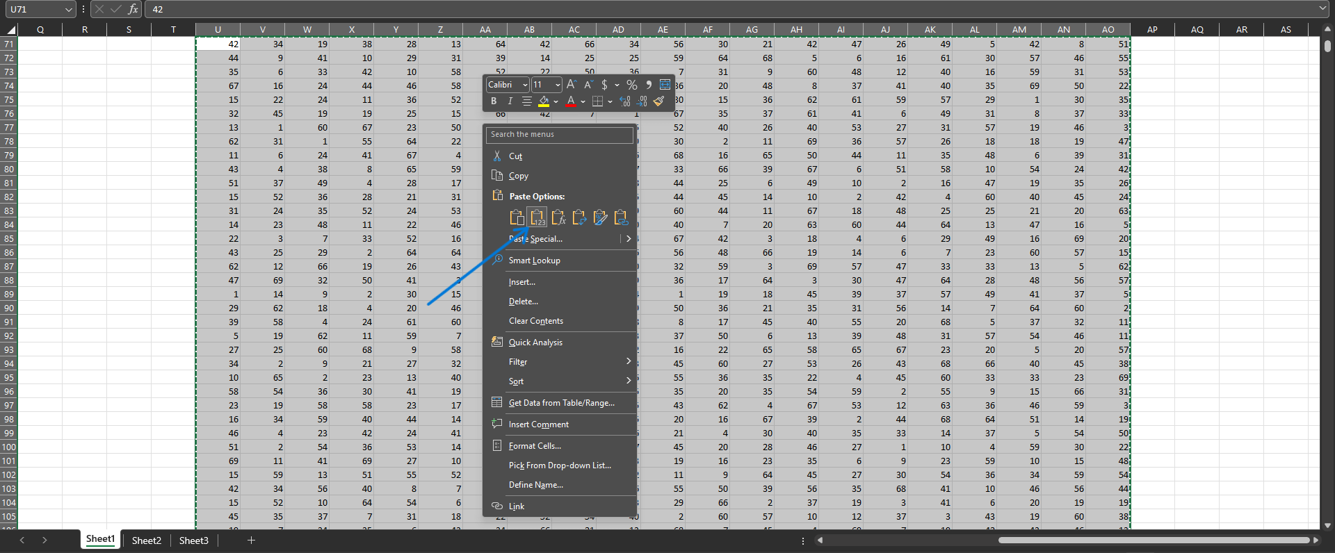
NOTE: The RANDBETWEEN function will continue to change the random combinations anytime you edit the sheet. This can disturb your calculation. To stop this, you should copy the entire combination and paste it again in order to overwrite the function and stop it.
Highlight the random lottery combinations by typing U71:AO6000 in the name box.
U71:AO6000
Copy it with “ CTRL + C”. After copying it, you should see dotted lines around the highlighted text.
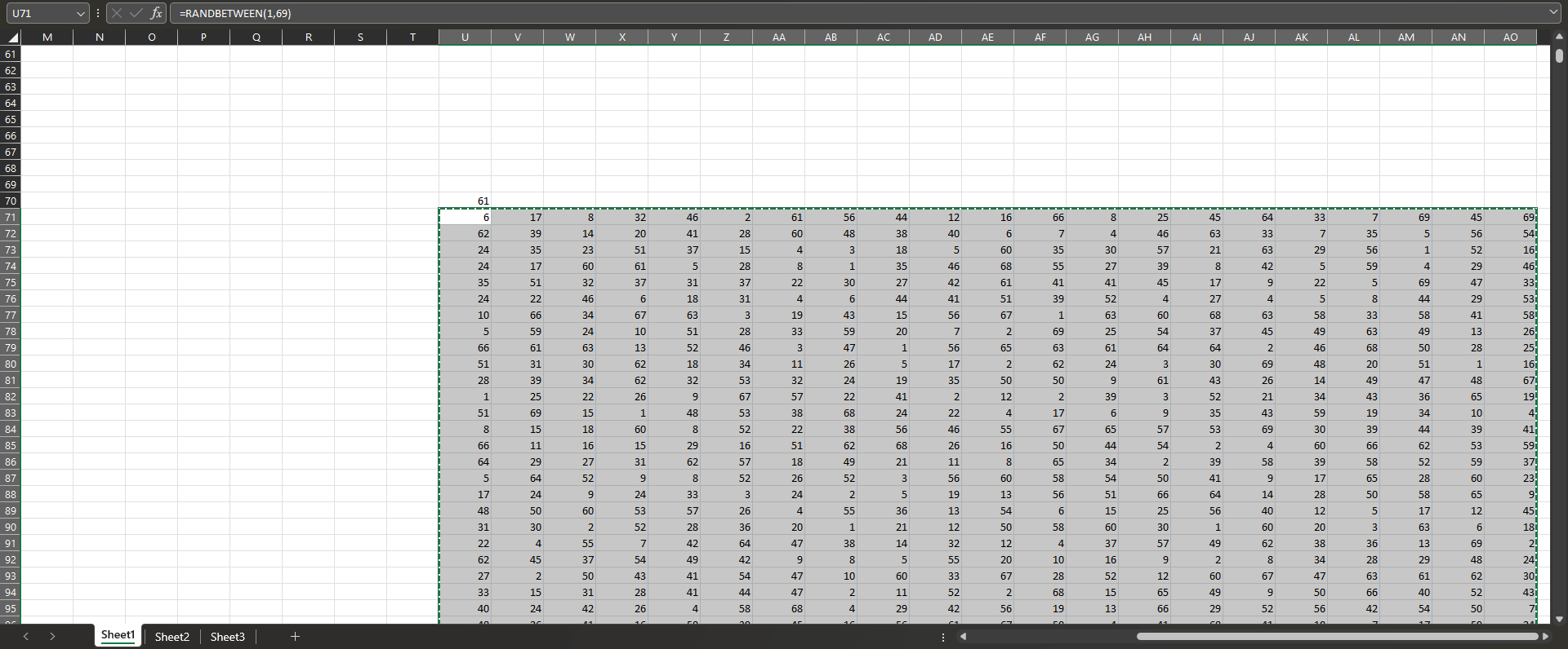
Right click immediately and click “PASTE SPECIAL VALUES”. This will overwrite the formula and keep the values constant.
Next, return to your B-row, and you’ll notice the workbook already counted how many times each number appears. Furthermore, it highlighted the cells with numbers that appear above average.
Repeat the Process by Using Only the Highlighted Numbers
The previous four steps used over 120,000 randomized numbers to select the most frequent ones and help you predict those to select on your ticket. You eliminated some numbers that remained below average, but you still have more than your ticket requires.
That’s why you want to run the process one more time. You can open a new document or use a new sheet within the same workbook. Either way, you need a blank sheet where you’d repeat the previous four steps.
The only difference is you won’t add all numbers from “1” to “69.” Instead, you want to use only the highlighted ones. There is no other way to do this, but manually, so you need to copy the values into the “A” row.
You’ll notice that our algorithm delivered 35 numbers above average. Next, enter the function in the B1 cell and copy it to the rest of the cells in the B range:
=COUNTIF($U$71:$AO$6000,A1)
Don’t forget the conditional formatting that should show the numbers above average clearly.
Expert tip: We didn’t want to change functions to avoid creating confusion. However, it’s perfectly fine to start U40 or any other cell apart from the already used ones. Please note that might change values required in other specified functions, too.
The next task is to enter the same function in U71:
=RANDBETWEEN(1,69)
And then, mark the cells “U71:AO6000” in the cell highlight box and enter that range. Copy the formula above to those cells. As you can see, it’s all the same as you did in the first workbook.
Here is our result (the numbers won’t be the same, but it should look like this):
Repeat the Process by Using Only the Highlighted Numbers
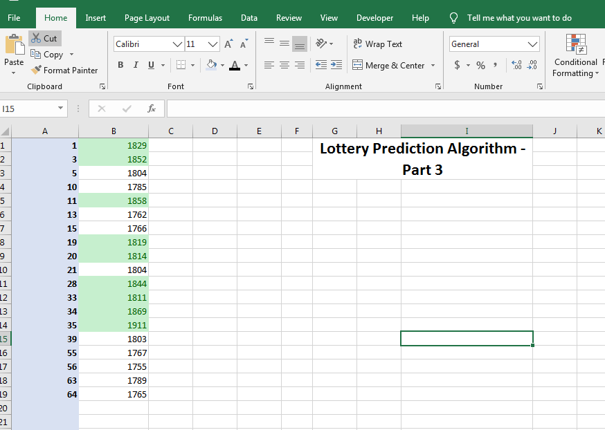
You can see that we still have too many numbers. That’s why we’ll repeat the process two more times:
The Final Selection
The third time we ran the numbers through the algorithm above, we got the following:
And finally, the fourth time we used the algorithm, we got our numbers for the upcoming Powerball round:
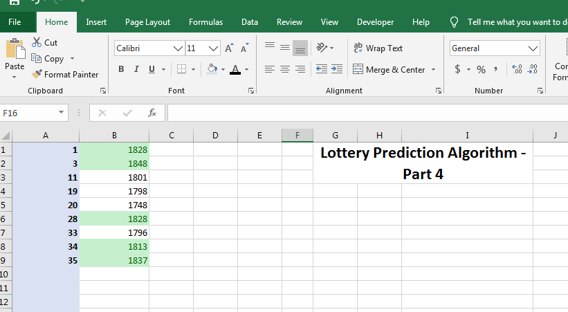
In our case, those are 1, 3, 28, 34, and 35.
It’s an excellent way to have fun in the process of selecting randomized numbers for your ticket. The odds of getting the same numbers are incredibly low. And the best part is that this algorithm applies to all lotteries. The only thing to consider is changing the numbers based on the lotto’s rules.
If you need some help creating the algorithm, you can check out our template for help. First make a copy of this sheet to make edits; then edit the first column to the required number pool in your lottery. Then creating random combinations with the steps highlighted in this guide.
After you generate your numbers, don’t forget to choose the best lottery sites to play your numbers. You can play on theLotter, Lotto Agent, WinTrillions, and Lottofy for a fantastic lottery experience.
Important Note We already listed the most recommended lottery sites, and you can also get some discounts. | ||
| GET 25% OFF for any ticket! | GET 20% OFF your first order, promo code: LOTTERYNGO | Buy 1 Ticket and Get 2 Tickets for FREE! |
Can You Determine Lottery Probability in Excel?
Yes, you can calculate lottery probabilities in Excel. Here is a quick guide on how to do that before a detailed explanation.
Create the following in your workbook:
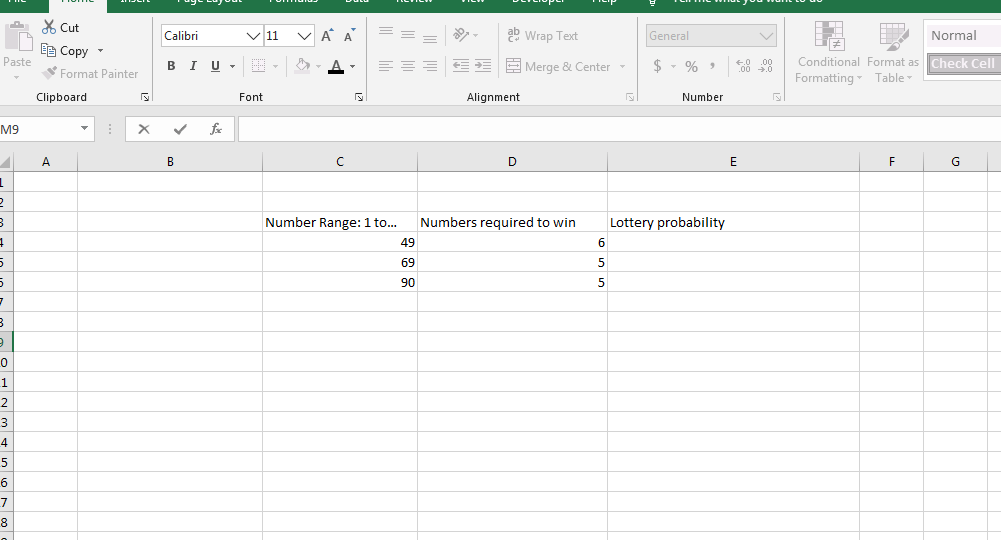
You can change the numbers based on the lottery you want to play. Next, in the E4 cell (or a suitable one in your workbook), type this function:
=COMBIN(C4, D4)
Use the little square in the bottom right corner of the E4 cell to copy the function to the bottom cells in the same row.
You’ll get the following:
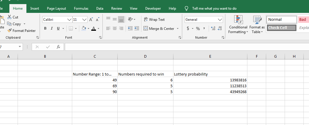
As you can see, the program calculated the odds of winning the 6/49 lottery as 13,983,816:1. If you analyze the Romania Lotto 6/49 that uses that concept, it shows the calculation is right. This could help you to compare the odds and see if investing the money for the ticket can be a smart move.
Can You Calculate the Probability of Two-Drum Lotteries in Excel?
You can also calculate the chances when you have a second drum included. For example, MegaMillions uses a 5/70 + 1/15 concept.
Here is how to calculate that – use the same table created for a single matrix and add these values:
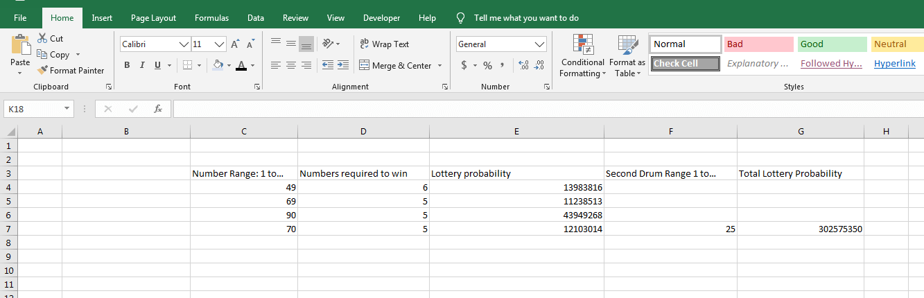
- Add 70 to the C7 or the corresponding cell for the number range.
- Add 5 for the numbers required to win (D7 or the corresponding cell).
- Use the function COMBIN(C7, D7) in the E7 cell to calculate the basic probability. Change the cell references if necessary.
- Add a second drum number range to the F7 cell (25 in case of MegaMillions).
- Add this function to the G7 cell “=E7*F7,” and you will notice the total lottery odds of winning the jackpot.
As you can see, it’s quite simple, and it can help you determine the grand prize-winning odds for any lottery in the world. If it seems easier, don’t hesitate to use our lottery odds calculator.
Important Note If you don’t have time to make your own lottery Excel prediction algorithm, you can always use our lottery predictor tool. We have already listed the most recommended lottery sites, and you can also get some discounts.
| ||
| GET 25% OFF for any ticket! | GET 20% OFF your first order, promo code: LOTTERYNGO | Buy 1 Ticket and Get 2 Tickets for FREE! |
Final Thoughts
Now you know how to use Microsoft Excel to create smart combinations for the upcoming lottery session. Lotto prediction algorithms are a fun and intriguing way to pick numbers for lottery tickets. These algorithms can analyze previous winning numbers, statistical probabilities, and other factors to generate a set of numbers that have a higher chance of being selected. It’s a fun and intriguing way to approach the lottery and who knows, it might even help you win!
Although they are completely random, it feels nice to conduct the process yourself. It also gives more confidence when you choose numbers with an algorithm that analyzes thousands of randomized number occurrences. Make sure to give this algorithm a shot, and who knows, those might be your lucky numbers!
When you are ready to play, do well to play with lottery sites like theLotter or Lotto Agent to get the best lottery experience.
FAQ
Are lottery prediction algorithms free to use?
The algorithm instructions on this page are completely free. By using them, you can create a prediction algorithm to predict the numbers for the upcoming lottery session.
Do lottery prediction algorithms guarantee a win?
No, these algorithms use the statistics based on large numbers to predict which ones to include on your ticket. However, everything is 100% random and doesn’t guarantee a win. Ultimately, the only way to win the lottery is to have enough luck.
How long does it take to create a lottery prediction algorithm?
It depends on how skilled you are with Excel. However, if you follow our guide, the entire process shouldn’t take more than 5-10 minutes.


")